This is a short monograph I wrote after finding a neat proof of a simple fact that I needed to know for my dissertation. It's too tedious and not relevant enough to go in the dissertation, but it is a neat application of real analysis to geometry. Therefore I decided to write it up very carefully, with a little bit of background. The intended audience is people who are interested in geometry and have seen some real analysis, but might not have much background aside from what you would see in a standard analysis course.
If you've taken a calculus class, you were probably taught at some point how to find the length of a smooth curve on the plane, which for now we'll call $C$.
There are four basic steps: first, you need to parameterize your curve, meaning find some smooth map $c: [a,b] \to \mathbb{R}^2$ which maps $[a,b]$ onto $C$. By this I mean, every point in $[a,b]$ needs to be mapped to a point in $C$, and every point in $C$ needs to be equal to $c(t)$ for some value $t$ in $[a,b]$. There are infinitely many different parameterizations of $C$, but it turns out that we can pick any of them and obtain the same length.
As a running example, I'm going to define a specific curve with a specific parameterization.
Let \[c(t) := (t - \frac{t^3}{3}, t^2),\] for $t \in [0,4]$.
Next, we need to calculate the derivative of $c$. By this, I mean that we need to calculate the derivatives of the components of $c$, giving us a new function $\dot{c}$. For the example function above, we have $\dot{c}(t) = (1 - t^2,2t)$. It is helpful to think of this as not just a vector in $\mathbb{R}^2$, but as a vector based at the point $c(t)$. This is because the significance of $\dot{c}(t)$ is that it is tangent to the curve $C$ at the point $c(t)$, and also tells us how fast and in which direction the parameterization is going through that point. To preserve this significance, we need to remember where $c(t)$ is. Usually, this point is skipped, and it isn't important mechanically for calculating the length of curves in the Euclidean plane, but it will be important later.
The next step is to calculate $\|\dot{c}(t)\|$, that is, the function that gives us the length of the vector $\dot{c}(t)$. Luckily, calculating the length of a vector in Euclidean space is easy: we simply apply Pythagoras's theorem to find \[\|\dot{c}(t)\| = \sqrt{\dot{c}_1(t)^2 + \dot{c}_2(t)^2}.\]
For our example function, this is $\sqrt{(1 - t^2)^2 + (2t)^2}$, which (after some arithmetic) is the same as $1 + t^2$.
The last step is to integrate $\|\dot{c}(t)\|$ over the interval $[a,b]$, which will tell us the length $L(C)$ of $C$. In the example, we get $\int_0^4 1 + t^2 dt = 4 + 64/3$.
This whole procedure is very mechanical. Why does it work? If you paid very close attention in calculus class, you might already know, but it's worth rehashing some of the particulars. Essentially, what we are doing is splitting up the interval $[a,b]$ into very small sub-intervals $[a,a + \frac{b-a}{N}], [a + \frac{b-a}{N},a+2\frac{b-a}{N}], \dots, [a+(N-1)\frac{b-a}{N},b]$. For each of the endpoints of these intervals, which we will denote $a_i^N := a + i \frac{b-a}{N}$, we place the point $c(a_i^N)$. Then, we connect the successive points together with straight lines. This produces an approximation $C^N$ of $C$ that is made up only of straight lines.
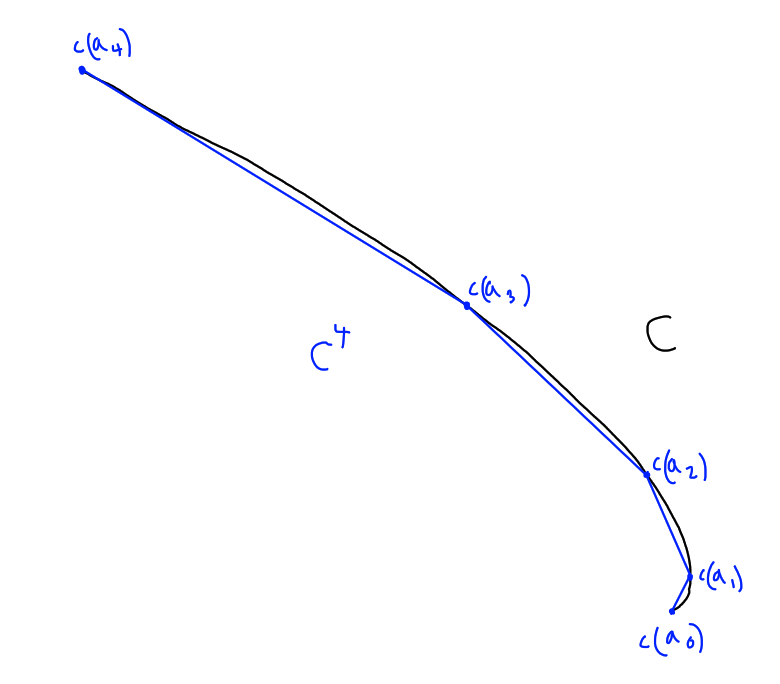
This is great! We can easily calculate the length of each of these straight lines, so we can easily calculate the length of this approximation: \[L(C^N) = \sum_{i = 1}^N \mathrm{dist}(c(a_{i-1}^N),c(a_i^N)).\]
$L(C^N)$ is an approximation of $L(C)$ essentially by definition. One way to justify this definition is to take as an axiom that straight line segments in Euclidean space are the shortest paths between their endpoints, so the length of the line segment connecting $c(a_{i-1}^N)$ to $c(a_i^N)$ is less than the length of the curve $c([a_{i-1}^N,a_i^N])$. Therefore $L(C^N)$ is always an under-estimate, and we define $L(C)$ to be the smallest value (if it exists) that is larger than $L(C^N)$ for all $N$. Equivalently, we could say \[L(C) := \sup_{N}\sup_{a = a_0 < a_1 < \dots < a_N = b}\sum_{i = 1}^N \mathrm{dist}(c(a_{i-1}),c(a_i)).\]
From now on, we'll drop the superscript $N$ and instead refer to one of these general subdivisions.
For each of the intervals $[a_{i-1},a_i]$, we know by the mean value theorem that there exists some point $\tilde{a}_i \in (a_{i-1},a_i)$ such that $\dot{c}(\tilde{a}_i) = \frac{c(a_i) - c(a_{i-1})}{a_i - a_{i-1}}$. Because the Euclidean distance between $c(a_{i-1})$ and $c(a_i)$ is simply given by $\|c(a_i) - c(a_{i-1})\|$, this tells us that \[L(C) = \sup \sum_i (a_i - a_{i-1})\|\dot{c}(\tilde{a}_i)\|.\]
Not so coincidentally, this is the same thing as the Riemann integral of the function $\|\dot{c}\|$ over the integral $[a,b]$, if it exists (why?). In this case, we know that our function at least has a continuous derivative, so this function is indeed integrable, and we arrive at our claimed fact, \[L(C) = \int_a^b \|\dot{c}(t)\| dt.\]
This is all well and good for curves in Euclidean space, but who says the Euclidean distance function is the only one? We could have substituted any distance function in for $\mathrm{dist}(a_{i-1},a_i)$ above. For instance, for someone traveling around the world, the distance between points on the surface of the Earth is what's relevant, not the distance between them on the map.
The distance function we pick needs to have a few basic properties. They are listed below:\[\begin{align*} \mathrm{dist}(x,y) \ge~ & 0\\ \mathrm{dist}(x,y) =~ & \mathrm{dist}(y,x)\\ \mathrm{dist}(x,y) =~ & 0 \text{ if and only if } x = y\\ \mathrm{dist}(x,y) \le~ &\mathrm{dist}(x,z) + \mathrm{dist}(z,y) \forall z \end{align*}\]
A function satisfying these properties is called a metric. It is only really relevant for our purposes to consider metrics on $\mathbb{R}^n$, but that does not mean we are restricted to the Euclidean metric. For instance, the popular taxicab metric could be used: $\mathrm{dist}_{\text{taxicab}}(x,y) := |x_1 - y_1| + |x_2 - y_2|$. One of the very curious things about the taxicab metric is that the length of the unit circle is equal to eight, rather than $2\pi$ as you might expect.
General metric spaces are interesting, but in some ways they are too general. For instance, nowhere in the definition do you see that this distance function is in any sense continuous; as I travel along a curve, the length can jump discontinuously. It also doesn't tell us that there is such a thing as a shortest path between two points.
What would be really useful is something like what we have for Euclidean space, where we were able to claim that $\mathrm{dist}(c(a_{i-1}),c(a_i)) = (a_i - a_{i-1})\|\dot{c}(\tilde{a}_i)\|$ for some number $\tilde{a}_i \in [a_{i-1},a_i]$. To make this work for metrics besides the Euclidean one, we need to first change the meaning of $\|\cdot\|$.
A pseudo-Finsler metric $\|\cdot\|$ on $\mathbb{R}^n$ is a function $\mathbb{R}^n \times \mathbb{R}^n \to \mathbb{R}$. The input $v_p$ refers to a vector $v \in \mathbb{R}^n$ based at the point $p \in \mathbb{R}^n$. A pseudo-Finsler metric has the following properties: \[\begin{align*} \|v_p\| &\ge 0 \forall v_p\\ \|\lambda v_p\| &= |\lambda| \|v_p\| \forall \lambda \in \mathbb{R}\\ \|\cdot\|~ & \text{is differentiable everywhere except possibly at}~ \{0_p: p \in \mathbb{R}^n\} \end{align*}\]
The first two assertions tell us that for each $p \in \mathbb{R}^n$, $\|\cdot\|$ is a norm on the space of vectors based at $p$, so it tells us coherently "how long" such vectors are. In fact, it defines a metric space structure on that vector space by setting $\mathrm{dist}_{\|\cdot\|}(v_p,w_p) = \|v_p - w_p\|$. The third assertion tells us that as the vector and the basepoint varies smoothly, the length also varies smoothly. With a few more restrictions on how smooth the metric is and what its derivatives can be, we would get the definition of a Finsler metric, which generalize Riemannian metrics. Those other properties aren't relevant for this document, though, so I won't go in to them here.
A metric space defined on $\mathbb{R}^n$ is a Finsler metric space if there exists a Finsler metric on $\mathbb{R}^n$ such that, for any continuously differentiable curve $c: [a,b] \to \mathbb{R}^n$ and any $\epsilon > 0$, there exists a number $\delta > 0$ such that, if $0 < t_2 - t_1 < \delta$, then \[|\|\dot{c}(\frac{t_1 + t_2}{2})\| - \frac{\mathrm{dist}(c(t_1),c(t_2))}{t_2 - t_1}| < \epsilon.\]
This condition essentially says that the Finsler metric $\|\cdot\|$ is the derivative of the length functional applied to any parameterized curve.
On a Finsler metric space, the same trick we applied earlier for turning the definition of length of a smooth curve in to an integral works. We must simply be careful about the supremums in a way we didn't need to before. In particular, we need to make sure that the subdivision $a_0 < a_1 < \dots < a_N$ we want to consider is such that $a_i - a_{i-1} < \delta$ for all $i > 0$. However, one thing we know by the definition of a metric space is that for any natural number $K$, \[\mathrm{dist}(c(a_{i-1}),c(a_i)) \le \sum_{j = 0}^{K-1} \mathrm{dist}(c(a_{i-1} + j\frac{a_i - a_{i-1}}{K}),c(a_{i} + (j+1)\frac{a_i - a_{i-1}}{2})).\]
So, for any subdivision $a = a_0 < a_1 < \dots < a_N = b$, we can always subdivide it more to obtain an approximation that is at least as long and satisfies $a_i - a_{i-1} < \delta$ for all $i$. So, any upper bound of the approximate lengths over all subdivisions satisfying this condition is also an upper bound of the approximate lengths over all subdivisions. Therefore the supremum can be calculated only using only subdivisions such that $a_i - a_{i-1} < \delta$ for all $i$.
By substituting the property of Finsler metric spaces in to the definition of the length of $C$, we get \[\begin{align*}L(C) &\le \sup_{a = a_0 < \dots < a_N = b} \sum_{i = 1}^N (a_i - a_{i-1})\left[\|\dot{c}(\frac{a_i + a_{i-1}}{2})\| + \epsilon\right]\\ &= \sup_{a = a_0 < \dots < a_N = b} \sum_{i = 1}^N (a_i - a_{i-1})\|\dot{c}(\frac{a_i + a_{i-1}}{2})\| + \epsilon(b - a)\\ &= \int_a^b \|\dot{c}(t)\|dt + \epsilon(b-a).\end{align*}\]
The last line is true by the definition of the integral. Since this was true for any $\epsilon > 0$, we get that $L(C) \le \int_a^b \|\dot{c}(t)\|dt$. We then get equality by taking any sequence of subdivisions such that $\lim_{N \to \infty}\max_{i} a_i - a_{i-1} = 0$ and noting that for this specific sequence of subdivisions, we get for all $\epsilon > 0$, \[\begin{align*}L(C) &\ge \lim_{N \to \infty} \sum_{i = 1}^N \mathrm{dist}(c(a_{i-1}),c(a_i)) \\ &\ge \lim_{N \to \infty} \sum_{i=1}^N (a_i - a_{i-1})\left[\|\dot{c}(\frac{a_i + a_{i-1}}{2})\| - \epsilon\right] \\ &= \int_a^b \|\dot{c}(t)\|dt - \epsilon(b-a).\end{align*}\]
This last equality is true because we asserted that $c$ is continuously differentiable and $\|\cdot\|$ is continuous. Otherwise, the length can fail to be Riemann integrable.
Note that, usually, the idea of a "Finsler metric space" is never defined, because you always get a canonical metric space from a Finsler metric, by setting $\mathrm{dist}(x,y) = \inf_{c}\int_a^b \|\dot{c}(t)\| dt$, where the infimum is over all continuously differentiable curves such that $c(a) = x$ and $c(b) = y$. However, in some cases you start out with a metric space structure and you need to show that there is a Finsler metric associated to it, like how we did in Euclidean space.
Now that we know the basic objects we're dealing with, I'd like to pose a problem.
Suppose $\|\cdot\|_1$ and $\|\cdot\|_2$ are two different Finsler metrics on $\mathbb{R}^n$, and let $L_1(C)$ be the length of $C$ measured in the $\|\cdot\|_1$ metric and likewise for $L_2$. What is $\sup_{C \subset \mathbb{R}^n} \frac{L_1(C)}{L_2(C)}$, where the supremum is taken over closed continuously differentiable curves in $\mathbb{R}^n$?
In order to keep some suspense, I'm not going to state the solution ahead of time. Instead, I'm going to work through the proof until we get to the answer.
Given any curve $C$, one thing we can do first to simplify the ratio $\frac{L_1(C)}{L_2(C)}$ is to first parameterize $C$ by its arc length in the $\|\cdot\|_2$ metric, so $c: [0,L_2(C)] \to \mathbb{R}^n$ traces out $C$ and $\|\dot{c}(t)\|_2 = 1$ for all $t$. Then, we can split up the length into lengths of small chunks $C^N_i := c([\frac{i-1}{N}L_2(C),\frac{i}{N}L_2(C)])$ of $C$: \[\frac{L_1(C)}{L_2(C)} = \frac{\sum_{i = 1}^{N} L_1(C^N_i)}{\sum_{i = 1}^{N} L_2(C_i^N)}\]
Since $c$ is a patameterization by $L_2$ arc length, it is true that $L_2(C_i^N) = \frac{L_2(C)}{N} = L_2(C_j^N)$ for any $i,j$. So, this sum simplifies: \[\frac{\sum_{i = 1}^N L_1(C_i^N)}{\sum_{i = 1}^N L_2(C_i^N)} = \sum_{i = 1}^N\frac{L_1(C_i^N)}{N L_2(C_i^N)} = \frac{1}{N} \sum_{i = 1}^N\frac{L_1(C_i^N)}{L_2(C_i^N)}.\]
So, the total ratio is equal to the average ratio over all of the chunks $C_i^N$. The average of any collection of numbers is always less than the maximum, so \[\frac{L_1(C)}{L_2(C)} \le \max_i \frac{L_1(C_i^N)}{L_2(C_i^N)}.\]
Since this is true for any $N$, it is certainly true in the limit as $N \to \infty$. In particular, we have \[\frac{L_1(C)}{L_2(C)} \le \limsup_{N \to \infty} \max_{i} \frac{L_1(C_i^N)}{L_2(C_i^N)}.\]
The next step is to expand out the lengths. On the top we have $L_1(C_i^N) = \int_{t_{i-1}}^{t_i} \|\dot{c}(t)\|_1 dt$, where $t_i := L_2(C)\frac{i}{N}$. On the bottom we have simply $L_2(C_i^N) = t_i - t_{i-1}$.
Since we assumed $C$ is continuously differentiable, $\dot{c}$ is continuous (and thus uniformly continuous) by definition, as is $\|\dot{c}\|_1$. Therefore there exists a number $\delta > 0$ such that if $t_{i} - t_{i-1} < \delta$, then $|\|\dot{c}(t)\|_1 - \|\dot{c}(\frac{t_{i-1} + t_i}{2})\|_1| < \epsilon$ for all $t \in [t_{i-1},t_i]$. This implies that \[\int_{t_{i-1}}^{t_i} \|\dot{c}(t)\|_1dt \le \int_{t_{i-1}}^{t_i} \left(\|\dot{c}(\frac{t_{i-1} + t_i}{2})\|_1 + \epsilon\right)dt = (t_i - t_{i-1})\left(\|\dot{c}(\frac{t_{i-1} + t_i}{2})\|_1 + \epsilon\right).\]
Plugging this back in to our main equality, and noting that as $N \to \infty$ all of the values $t_i - t_{i-1}$ will become less than any fixed number $\delta > 0$, we get that for any $\epsilon > 0$, \[\frac{L_1(C)}{L_2(C)} \le \limsup_{N \to \infty} \max_i \frac{(t_i - t_{i-1})\left(\|\dot{c}(\frac{t_{i-1} + t_i}{2})\|_1 + \epsilon\right)}{t_i - t_{i-1}} = \limsup_{N \to \infty} \max_i \|\dot{c}(\frac{t_{i-1} + t_i}{2})\|_1 + \epsilon.\]
Since this was true for any $\epsilon > 0$, it must be true that $\frac{L_1(C)}{L_2(C)} \le \limsup_{N \to \infty} \max_i \|\dot{c}(\frac{t_{i-1} + t_i}{2})\|_1$.
Note that for any fixed $K \ge 0$, the set $\{a + \frac{2i + 1}{2N}L_2(C): N > K, 0 \le i \le N-1\}$ is dense in $[a,b]$. Since this is exactly the set of points that $\|\dot{c}\|_1$ is being evaluated over in the limsup, and $\|\dot{c}\|_1$ is continuous on $[a,b]$, this implies \[\limsup_{N \to \infty} \max_i \|\dot{c}(\frac{t_{i - 1} + t_i}{2})\|_1 = \sup_{t \in [a,b]} \|\dot{c}(t)\|_1 = \sup_{t \in [a,b]} \frac{\|\dot{c}(t)\|_1}{\|\dot{c}(t)\|_2}.\]
We're essentially done. The next step is to notice that $\dot{c}(t)$ is a nonzero vector based at $c(t)$. So, certainly $\frac{\|\dot{c}(t)\|_1}{\|\dot{c}(t)\|_2} \le \sup_{v_p \ne 0_p} \frac{\|v_p\|_1}{\|v_p\|_2}$, and we get \[\frac{L_1(C)}{L_2(C)} \le \sup_{v_p \ne 0_p} \frac{\|v_p\|_1}{\|v_p\|_2}.\]
Our task now is to get the reverse bound. Let ${v_i}_{p_i}$ be a sequence of nonzero vectors such that $\lim_{i \to \infty} \frac{\|{v_i}_{p_i}\|_1}{\|{v_i}_{p_i}\|_2} = \sup_{v_p \ne 0_p} \frac{\|v_p\|_1}{\|v_p\|_2}$. For each $i$, let $\gamma_i: [0,1] \to \mathbb{R}^n$ be a smooth curve such that $\gamma_i(0) = p_i$, $\dot{\gamma}_i(0) = \frac{{v_i}_{p_i}}{\|{v_i}_{p_i}\|_2}$, and $\gamma_i$ is parameterized by its $\|\cdot\|_2$ arc length. Such a curve could be found, for instance, by taking the curve $\hat{\gamma}_i(t) = p_i + t {v_i}_{p_i}$ for $t \in [0,\infty)$, reparameterizing it by its $\|\cdot\|_2$ arc length, and then restricting to the interval $[0,1]$.
We already know that $L_1(\gamma_i([0,\delta])) = \int_0^\delta \|\dot{\gamma}_i(t)\|_1dt$ for any $\delta > 0$. We also know that, because $\dot\gamma_i$ is continuous, for any $\epsilon > 0$ there exists a value $\delta_i(\epsilon) > 0$ such that if $t < \delta_i(\epsilon)$, then $| \|\dot\gamma(t)\|_1 - \|\dot{\gamma}(0)\|_1 | < \epsilon$. Therefore, we have \[\begin{align*} \frac{\|{v_i}_{p_i}\|_1}{\|{v_i}_{p_i}\|_2} = \|\dot{\gamma}(0)\|_1 &= \frac{\delta_i(\epsilon) \|\dot{\gamma}(0)\|_1}{\delta_i(\epsilon)} \\ &\le \frac{\int_0^{\delta_i(\epsilon)} \|\dot{\gamma}_i(0)\|_1dt}{\delta_i(\epsilon)}\\ &\le \frac{\int_0^{\delta_i(\epsilon)} \left(\|\dot{\gamma}_i(t)\|_1 + \epsilon\right)dt}{\delta_i(\epsilon)}\\ &= \frac{L_1(\gamma_i([0,\delta_i(\epsilon)]))}{L_2(\gamma_i([0,\delta_i(\epsilon)]))} + \epsilon \end{align*}\]
So, taking $C_i^\epsilon = \gamma_i([0,\delta_i(\epsilon)])$, \[\sup_{v_p}\frac{\|v_p\|_1}{\|v_p\|_2} = \lim_{i \to \infty} \frac{\|{v_i}_{p_i}\|_1}{\|{v_i}_{p_i}\|_2} \le \lim_{i \to \infty} \frac{L_1(C_i^\epsilon)}{L_2(C_i^\epsilon)} + \epsilon \le \sup_C \frac{L_1(C)}{L_2(C)} + \epsilon.\]
This was true for any $\epsilon > 0$, so it is true that $\sup_{v_p \ne 0_p} \frac{\|v_p\|_1}{\|v_p\|_2} = \sup_C \frac{L_1(C)}{L_2(C)}$. $\Box$
And there we have it: the supremum of the ratio between the lengths of continuously differentiable curves measured by two Finsler metrics is equal to the supremum of the ratio between the lengths of vectors measured by those Finsler metrics. While not exactly surprising, a full non-handwave proof required some proper real analysis. It's also a useful result, since directly bounding the ratio between lengths of curves is nigh impossible compared to bounding the ratio between lengths of vectors.